Loan Default Project

Business Objective

A bank has given us a data set and would like us to find which potential customers will likely repay a bank loan and what questions to ask on future applications based off of previous loan data.

Data set of Loans and if they were paid or defaulted.
Look for the Customers who have paid and predict if future customers will pay back or default loan.
Come up with questions for customer when they are applying for loan

import pandas as pd

df = pd.read_csv('1533148983_LoansTrainingSet.csv')

Taking a Look at the Data

df.info()

<class 'pandas.core.frame.DataFrame'>
RangeIndex: 256984 entries, 0 to 256983
Data columns (total 19 columns):
Loan ID                         256984 non-null object
Customer ID                     256984 non-null object
Loan Status                     256984 non-null object
Current Loan Amount             256984 non-null int64
Term                            256984 non-null object
Credit Score                    195308 non-null float64
Years in current job            245508 non-null object
Home Ownership                  256984 non-null object
Annual Income                   195308 non-null float64
Purpose                         256984 non-null object
Monthly Debt                    256984 non-null object
Years of Credit History         256984 non-null float64
Months since last delinquent    116601 non-null float64
Number of Open Accounts         256984 non-null int64
Number of Credit Problems       256984 non-null int64
Current Credit Balance          256984 non-null int64
Maximum Open Credit             256984 non-null object
Bankruptcies                    256455 non-null float64
Tax Liens                       256961 non-null float64
dtypes: float64(6), int64(4), object(9)
memory usage: 37.3+ MB

df.head()

	Loan ID	Customer ID	Loan Status	Current Loan Amount	Term	Credit Score	Years in current job	Home Ownership	Annual Income	Purpose	Monthly Debt	Years of Credit History	Months since last delinquent	Number of Open Accounts	Current Credit Balance	Maximum Open Credit
0	000025bb-5694-4cff-b17d-192b1a98ba44	5ebc8bb1-5eb9-4404-b11b-a6eebc401a19	Fully Paid	11520	Short Term	741.0	10+ years	Home Mortgage	33694.0	Debt Consolidation	$584.03	12.3	41.0	10	6760	16056
1	00002c49-3a29-4bd4-8f67-c8f8fbc1048c	927b388d-2e01-423f-a8dc-f7e42d668f46	Fully Paid	3441	Short Term	734.0	4 years	Home Mortgage	42269.0	other	$1,106.04	26.3	NaN	17	6262	19149
2	00002d89-27f3-409b-aa76-90834f359a65	defce609-c631-447d-aad6-1270615e89c4	Fully Paid	21029	Short Term	747.0	10+ years	Home Mortgage	90126.0	Debt Consolidation	$1,321.85	28.8	NaN	5	20967	28335
3	00005222-b4d8-45a4-ad8c-186057e24233	070bcecb-aae7-4485-a26a-e0403e7bb6c5	Fully Paid	18743	Short Term	747.0	10+ years	Own Home	38072.0	Debt Consolidation	$751.92	26.2	NaN	9	22529	43915
4	0000757f-a121-41ed-b17b-162e76647c1f	dde79588-12f0-4811-bab0-e2b07f633fcd	Fully Paid	11731	Short Term	746.0	4 years	Rent	50025.0	Debt Consolidation	$355.18	11.5	NaN	12	17391	37081

Going through each column, duplicate values have been recorded, missing information needs to be filled in multiple columns and object columns need to be convereted to numbers. Also, the ‘credit score’ column has a recording error. The column most important column we need for analysis is ‘Loan Status’. Which is our column that shows if a loan was paid off or defaulted.

# drop exact duplicate rows 
df.drop_duplicates(keep='first', inplace=True)

# Split Columns between numbers and objects to groupby 'Loan ID' so we can fill in missing values
df_obj = df.select_dtypes(include='object')
df_num = df.select_dtypes(exclude='object')

# Loan ID to numbers data frame so can use groupby
df_num['Loan ID'] = df['Loan ID']

# groupby Loan ID and takes the max of each loan
df_num = df_num.groupby('Loan ID').max().reset_index()
df_obj = df_obj.drop_duplicates(subset='Loan ID')
df = df_obj.merge(df_num) 

# grabbing Loan and Customer ID
loan_cust_id = df[['Loan ID', 'Customer ID']]
df.drop(['Loan ID', 'Customer ID'], axis=1, inplace=True)

Filling in Missing Data

Columns with NaN values were filled with values similar to data in the row

# BANKRUPTCIES
df['Bankruptcies'].fillna(0.0, inplace=True)
df['Tax Liens'].fillna(0.0, inplace=True)
# Months since last delinquent
df['Months since last delinquent'].fillna(0.0, inplace = True)
# Replace Column Years in current job == < 1 Year to .5 integer
df['Years in current job'].replace('< 1 year', 0.5, inplace=True)
# Replace Column Years in current job == 10+ Year to 15 year
df['Years in current job'].replace('10+ years', '15 year', inplace=True)
# Fill NaN Values in Years in current job column to '0 year' string
df['Years in current job'] = df['Years in current job'].fillna(value='0 years')
# Extracts digit from Years in current job and changes Years in current job to int
df['Years in current job'] = df['Years in current job'].str.extract('(\d+)').astype(float)
# Fill NaN Values in Years to 0.5 for < 1 year
df['Years in current job'] = df['Years in current job'].fillna(value=0.5)

CORRECTING DATA INPUT ERRORS

# replace other to Other
df.replace('other', 'Other', inplace=True)
# Changes #VALUE! in Maximum Open Credit to 0
df.loc[df['Maximum Open Credit'] == '#VALUE!', 'Maximum Open Credit'] = df['Current Loan Amount'].median()
# found median of Loan Amount without the 99999999 values
loan_median = df[df['Current Loan Amount'] < 99999999]['Current Loan Amount'].median()
# Change the 9999999 Loan Amount Values to loan median
df.loc[df['Current Loan Amount'] == 99999999, 'Current Loan Amount'] = loan_median
# replace HaveMortgage to Home Mortgage
df.replace('HaveMortgage', 'Home Mortgage', inplace=True)

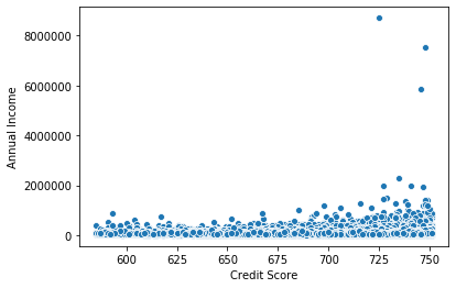
For a score with a range between 300-850, a credit score of 700 or above is generally considered good. A score of 800 or above on the same range is considered to be excellent. Most credit scores fall between 600 and 750

df['Credit Score'].describe()

count    171202.000000
mean       1261.776013
std        1775.229972
min         585.000000
25%         716.000000
50%         735.000000
75%         745.000000
max        7510.000000
Name: Credit Score, dtype: float64

df['Credit Score'] = df['Credit Score'].apply(lambda x : x / 10 if x > 1000 else x)

df['Credit Score'].describe()

count    171202.000000
mean        722.755698
std          26.827283
min         585.000000
25%         712.000000
50%         732.000000
75%         742.000000
max         751.000000
Name: Credit Score, dtype: float64

Changing Object Columns to numeric

Many of the columns have object data types including: Term, Home Ownership, Purpose, Loan Status, Monthly Debt and Maximum Open Credit. Those that will be changed to nonordinal datatype include Term, Home Ownership, Purpose. The other columns will be changed to numerical. Loan Status, which is our target, will be converted to 0 based on being paid off and 1 being unpaid.

d = {'Fully Paid': 0, 'Charged Off': 1}
df['Loan Status'] = df['Loan Status'].map(d)

# removing , and $ from Monthly Debt and changing to float
df['Monthly Debt'] = df['Monthly Debt'].str.replace(',','')
df['Monthly Debt'] = df['Monthly Debt'].str.replace('$','')
df['Monthly Debt'] = df['Monthly Debt'].astype(float)

df['Maximum Open Credit'] = df['Maximum Open Credit'].astype(float)

Creating Dummies for the Columns: Term, Home Ownership and Purpose

df = pd.get_dummies(df, drop_first=True)

loan = df.corr()['Loan Status']

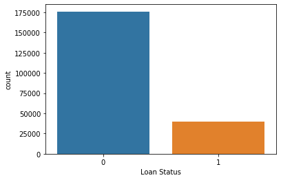
sns.countplot(x='Loan Status', data=df)

png

sns.scatterplot(x='Credit Score', y='Annual Income', data=df)

png

# Take out Loan Status and Annual Income to predict them
loan_status = df['Loan Status']
income = df['Annual Income']
df.drop(['Loan Status', 'Annual Income'], axis=1, inplace=True)

from sklearn.linear_model import LinearRegression
from sklearn.model_selection import train_test_split
from sklearn.metrics import r2_score, mean_squared_error

filled = df[df['Credit Score'].notnull()]
missing = df[df['Credit Score'].isnull()]

X_train, X_test, y_train, y_test = train_test_split(filled.drop('Credit Score', axis=1), 
                                                    filled['Credit Score'], test_size=0.4, random_state=101)

L = LinearRegression()

L.fit(X_train, y_train)

r2_score(y_train, L.predict(X_train))

0.28462988125672517

mean_squared_error(y_train, L.predict(X_train))**.5

22.740334260998736

predict = L.predict(X_test)

predictions = L.predict(missing.drop('Credit Score', axis=1))

missing['Credit Score'] = predictions
df = pd.concat([missing, filled])

# Adding Annual Income Column back
df['Annual Income'] = income

filled = df[df['Annual Income'].notnull()]
missing = df[df['Annual Income'].isnull()]

X_train, X_test, y_train, y_test = train_test_split(filled.drop('Annual Income', axis=1), 
                                                    filled['Annual Income'], test_size=0.4, random_state=101)

L.fit(X_train, y_train)

print(r2_score(y_test, L.predict(X_test)))
print(mean_squared_error(y_test, L.predict(X_test))**.5)

0.3833735024596715
38215.97609792463

prediction = L.predict(missing.drop('Annual Income', axis=1))
missing['Annual Income'] = prediction

df = pd.concat([missing, filled])

df['Loan Status'] = loan_status

sns.countplot(x='Loan Status', data=df)

png

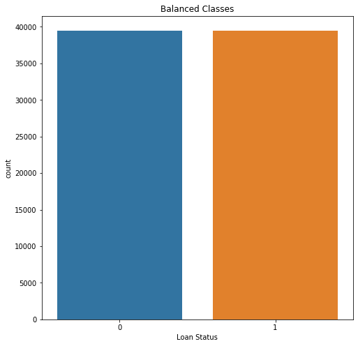
Imbalanced Data

Using undersampling to balance out the number of Loans that were paid off and unpaid. The under sampled ‘Loan Status’ which is the charged off loans will match the number of paid off loans.

# Shuffle the Dataset.
shuffled_df = df.sample(frac=1,random_state=4)

# Put all the charged off loan class in a separate dataset.
upaid_df = shuffled_df.loc[shuffled_df['Loan Status'] == 1]

#Randomly select 492 observations from the paid off (majority class)
paid_df = shuffled_df.loc[shuffled_df['Loan Status'] == 0].sample(n=39509,random_state=42)

# Concatenate both dataframes again
normalized_df = pd.concat([upaid_df, paid_df])

#plot the dataset after the undersampling
plt.figure(figsize=(8, 8))
sns.countplot('Loan Status', data=normalized_df)
plt.title('Balanced Classes')
plt.show()

png

X = normalized_df.drop('Loan Status', axis=1)
y = normalized_df['Loan Status']
X_train, X_test, y_train, y_test = train_test_split(X, y, test_size=0.4, random_state=101, 
                                                    stratify=normalized_df['Loan Status'])

from sklearn.linear_model import LogisticRegression
log = LogisticRegression()

log.fit(X_train, y_train)

LogisticRegression(C=1.0, class_weight=None, dual=False, fit_intercept=True,
                   intercept_scaling=1, l1_ratio=None, max_iter=100,
                   multi_class='auto', n_jobs=None, penalty='l2',
                   random_state=None, solver='lbfgs', tol=0.0001, verbose=0,
                   warm_start=False)

predictions = log.predict(X_test)

from sklearn.metrics import classification_report, confusion_matrix

print(classification_report(y_test, predictions))

              precision    recall  f1-score   support

           0       0.59      0.60      0.60     15804
           1       0.60      0.59      0.59     15804

    accuracy                           0.59     31608
   macro avg       0.59      0.59      0.59     31608
weighted avg       0.59      0.59      0.59     31608

Based off the classification report, we scored about 60% accuracy that people will both pay back their loans and if they will default on their loans.

import numpy as np   

feature_importance = abs(log.coef_[0])
feature_importance = 100.0 * (feature_importance / feature_importance.max())
sorted_idx = np.argsort(feature_importance)
pos = np.arange(sorted_idx.shape[0]) + .5

featfig = plt.figure()
featax = featfig.add_subplot(1, 1, 1)
featax.barh(pos, feature_importance[sorted_idx], align='center')
featax.set_yticks(pos)
featax.set_yticklabels(np.array(X.columns)[sorted_idx], fontsize=8)
featax.set_xlabel('Relative Feature Importance')

plt.tight_layout()   
plt.show()

png

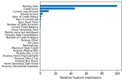
Conclusion

After looking at the chart above which feature importance that is based off of the column coefficients, the most important questions to ask future loan applicants are:

How much is their monthly debt?
What is their credit score?
How much is their current loan amount?
What is their annual income?

Share on

Twitter Facebook LinkedIn

Victor Chen